
Rob Dymond-Green, Technical Manager for the UK Data Service Census Support Service, describes the creation and processing of the 2011 UK Census dataset, available through InFuse.
As far as we know, the dataset we have created as part of processing the 2011 UK Census data is unique as it combines data from the Office of National Statistics (ONS) which produces data for England and Wales, the National Records Scotland (NRS) which produce data for Scotland, and the Northern Ireland Statistics and Research Agency (NISRA) which produces data for Northern Ireland. The three census agencies provide coverage across the UK, where these censuses were subject to their distinctive characteristics necessitated by the requirement to create outputs tailored to their own audiences. The work we have done consisted in unpicking these characteristics – creating a consistent dataset which enables the thousands of users of the data to perform novel analyses across all geographies in the UK – saving them hours of work; resulting in significant efficiencies.
The unified description describes the data as well as the geographies, as one interrelated whole, which enables users to query the data in ways that have not been possible in the past, or have been really difficult and time consuming. For example, you can find out how often ‘Age 0 to 4’ is used and if this code is used with other combinations of codelists and codes; you can also find out the geographic coverage of the variable in terms of the extent and the geographic granularity. Conversely you can pick a geographic level or area and find out what data is available for it.

Image credit: https://unsplash.com/
Why have we re-described the 2011 UK Census?
A big issue with the 2011 Census was that similar information was published across multiple tables but was described differently, due to the way the table was originally commissioned for a particular audience. As a user it meant that you had to grapple with sifting through the meaning to see if the tables were describing the same concept; you had to first find a table by its title – that sounded like it contained the information you wanted, then you had to open it and see if it contained the particular combination of variables that you were interested in. This repeated search and manual normalisation exercise was time-consuming and our users used to provide feedback saying they were never quite sure if they had identified all tables with the information they wanted.
Justin Hayes, Census support Manager tells us:
“So we thought that there must be a better way. Could the metadata be made consistent where all the things that are about the same concept are grouped together into topics, such as ‘age’ or ‘ethnicity’ and could the labels for variables within these topics be normalised? We looked around to see if there were standards that could be applied to the 2011 Census metadata which would enable this grouping and normalisation approach and we identified 2 possibilities: DDI and SDMX.”
When we evaluated DDI 3.1, we discovered that it could describe the structure needed, but we identified an issue with describing the geography. It had the capability to describe the complexity of the UK geographic hierarchy, but was extremely verbose and introduced lots of duplication in the way that it recorded the interaction between parent-child relationships. At the time of our research, it was not possible to describe a relationship where a child geography had multiple parents. Each object in the geographic schema in DDI needs to be unique, so to be able to describe the multiple parent scenario, we would have had to duplicate each child. A key requirement for our system was to enable the multiple parent model for geography, giving our users the ability to pick all child areas of a type for a given parent. For a simple hierarchy, that wouldn’t be too much of an issue but when you are dealing about 10,000 middle super output areas and you need to describe the relationship to each of the output areas they have as children where there are 230,000 output areas. Then separately describing the 30,000 lower super output areas and their child output areas, this duplication soon adds up. Then separately, we would have had to use a comparability schema (which DDI has) to then describe the multiple occurrences of each of the output areas to say that they were equivalent, we’d need to do this for all the other areas which had to be duplicated further up the hierarchy.
When we looked at SDMX, it too contains the structure that would be needed to describe concepts and topics. It also has a concept of geography, but more importantly it has the ability to describe multiple parents, thus removing the duplication that DDI required. So we decided to use this for our core model, although part of this decision was influenced by the need for the ONS to produce outputs from the 2011 Census in SDMX for a Eurostat project attempting to create a hub of consistent 2011 Census data across Europe.
How we processed the data
We started by processing data from the ONS, as the majority of our historic use is England and we wanted to release data to our users as soon as possible. The earlier releases of ONS data was their ‘simpler’ tables which contained data about a single topic or groups of topics along a theme, such as employment, and this data formed our initial release. We then moved onto processing the more complicated multi-topic tables (tables that can contain up to 6 topics as cross tabulations, e.g. Age By Region By Sex), which were published as our second release. Afterwards we moved on to the more trickier job of matching data from Northern Ireland and Scotland for our third release.
Table 1: Number of source tables by census agency that have been processed to create the 2011 UK Census dataset
| Agency | Number of Census Tables |
| Office of National Statistics | 693 |
| National Records Scotland | 411 |
| Northern Ireland Statistics and Research Agency | 512 |
| Total | 1616 |
Given that we started processing data from England and Wales first, we based all topics and labels on those data and then matched each new Census table into this set, making changes where needed and adding new items if the particular topic or label didn’t exist. This process has produced a set of 171 topics, containing 4,928 labels, and 934 topic combinations (topic cross tabulations). Details about how each type of Census table has been processed and about the matching process is described later in the blog.
As you can see in Table 2 below, the ONS data was pretty clean and only required changes to 20.5% of the labels, whereas for NISRA 64.63 % was changed and for NRS 79.75%.
Table 2: Degree of textual changes made to the raw data
| Agency | Cells* | Raw text descriptions | Additions (Universe and Units) | Matched raw text | Change to raw labels | % change |
| ONS | 188,431 | 611,144 | 300,639 | 485,796 | 125,348 | 20.51 |
| NISRA | 142,372 | 438,471 | 248,933 | 155,052 | 283,419 | 64.63 |
| NRS | 54,300 | 152,965 | 123,539 | 30,967 | 121,998 | 79.75 |
In Table 2 we added some more information in the form of Universe and Units, which are concepts to describe all aspects of the Census dataset being processed, as we had feedback through user support queries that sometimes our users were confused by these, so we decided to be as explicit as we could be when describing the datasets.
The result of all this matching work is a more consistent dataset, where the same concepts are coded the same. This enables us to show our end users what data that is available across countries. The table below shows the combinations of countries where we have comparable data cells.
Table 3: Combinations of countries with comparable data cells
| Coverage | Number of Cells* |
| England, Wales | 158,447 |
| Northern Ireland | 133,781 |
| Scotland | 43,791 |
| Wales | 11,393 |
| England, Scotland, Wales | 5,874 |
| England, Northern Ireland, Scotland, Wales | 4,209 |
| England, Northern Ireland, Wales | 2,555 |
| Northern Ireland, Scotland | 1,053 |
| England | 152 |
*In this instance a cell is basically an ID that has been given to a group of concepts that describes the item being measured, for instance people aged 3 and over, or something a bit more complicated like people in employment who work part time who work in the healthcare industry and are English and Muslim.
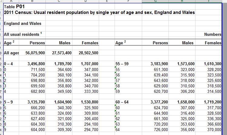
As I previously mentioned, each of the census agencies in the UK produce and publish this data in different ways and it comes in a variety of formats: text, Excel and PDF files. Even an individual census agency may publish the data using different formats. For instance, the first set of results for 2011 was published by the ONS as a set of Excel tables. These tables were created manually and were designed to be visually pleasing and easy to read (as shown in Figure 1 below).
Figure 1: Cross table of Age by Sex for England and Wales
To be able to load this into the SDMX model we had to define the concepts, codelists and codes used. As we use SDMX, we changed the nomenclature used (for a topic we use the term Codelist and for a label we use the term Code.
For example, in the case of the Table P01 (Fugure 1), mapping the concepts, codelists and codes used is pretty easy as we have the concepts of Age (single years), Sex, and the unit and the universe, although within our model we broke up the universe to enable cross search within the data structure (cube).
To process this particular table we add a consistent column name ID (a cell ID). To ensure consistency with other tables, we follow the schema where we use a table prefix that is the table ID, followed by 1 to n, where n is the number of columns in the table. This then creates an ID that will be unique within the system, we can then attach the codes and codelists values to this new, unique cell ID. Looking at the table we can take an educated guess that the columns which contain Males are part of a Sex codelist, so we can create this codelist if it doesn’t already exist in our library of codelists and add Males to this codelist if it doesn’t exist either. Likewise we can make the assumption that the rows beginning with All Ages contains codes for an age codelist. Using the information from the table name, we can deduce that it’s not a special version of age, as labels for age could be used in more than one concept, e.g. Age of Household reference person, Age at arrival into the UK. The Age column also has a footnote attached to it, so we can use this information to help us inform what codelist it could be applied to.
Again, if the labels (codes) for each age listed are not present in the Age codelist, we would add them. This codelist also looks like it could be hierarchical as there is a label of 0 – 4 followed by rows showing 0, 1, 2, 3, and 4. We would define this relationship, this would then alter our working model of how this data is described, because based on the name of the codelist listed in the table title it should only contain single ages. At this point we would need to make a value judgement between describing the data as listed versus the utility of having a single codelist for the Age variable; In InFuse we decided to err on the utility side, so we have a single codelist for Age.
Figure 2: Cross table of Age by Sex for local authorities
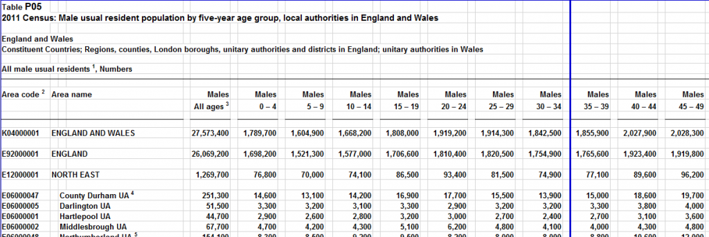
As you can see from the example above, we have another table which contains data for Age by Sex, however this time it has data to a finer granularity in terms of areas covered as it has data at the local authority level. Again, we can use the table title to help us to work out what codelists this table contains. As we have a single codelist for Age we can then apply the codes that we created earlier when we described table P01 for Age and also for Sex. The implication of the decisions that we made is that we have now grouped the data from Tables P01 and P05 together (as they are described using the same set of codelists and codes). This means that our users can pick Age by Sex and see all the data in one place.
As we continue to process additional tables, our working model for the description of the data changes and evolves. Assumptions we have made based on the data we have processed so far may change and we would then need to work back through the data tables previously described to check that the proposed changes don’t end up misrepresenting the data.
Figure 3: Marital and civil partnership status by Age
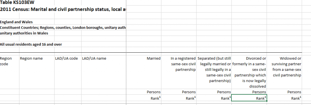
So for the table above we would have a Marital and Civil Partnership status codelist, but as we describe the universe we would add 16 and over to the Age codelist.
Figure 4: Living arrangements by Age by Resident type
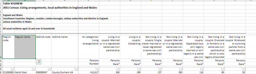
To process this table we have a choice to make, because we can either add this as a new codelist called Living Arrangements or if we look at the label used, we see that actually it is also describing Marital and Civil Partnership status. So an alternative description for this table could be Couple Status by Marital and Civil Partnership status by Age by Resident type (the resident type bit has come from the universe as this table is a subset consisting of people who live in households, rather than a count of all usual residents).
For these types of tables, all the information needed to decide how they are described is within the same excel file, this is not the case for all the outputs produced. For later ONS releases, they use a different format and split the data and metadata, the metadata information was supplied in 2 separate files per data table, one file contained the cell description as a comma separated list and the other contained information about the table universe.
Figure 5: Example csv description file
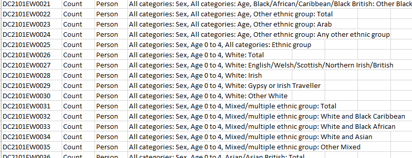
In Figure 5 above, we have a file which is more computer readable, however because we created our working model based on Releases 1 and 2, we find that the labelling that has been used to describe the same codes can be different, so this data needs to be matched manually. For instance, in the earlier examples the age codes were labelled 0 – 4, but the new age label format used in this multivariate data is labelled as Age 0 to 4. For a human, it is easy to see that’s it’s the same thing but not for a computer, which means this matching to the pre-existing code has to be a manual process. The other issue that crept in between Releases 1, 2 and the following releases was that the topic names used in the table names was not consistent, so we couldn’t reliably use this as way to work out if we had already captured this information.
Because this is a manual process, Jamey Hart, Data Quality Officer on the team, had to do rigorous Quality Assurance (QA) to check that our ‘normalised’ description of each table had captured the essence of what the published table contained. This included eyeballing our description of the table and comparing this to the original supplied version. Jamey continues:

“We worked through approximately 140,000 cells at this stage. The reason for the rigorous QA was that we now have a consistent set of descriptions and we have ensured that the same concepts are described in the same way – and we can begin to de-duplicate the data so that we only hold one version of a particular data item (cell). This de-duplication process also takes into account the geographic extent of the cell and its granularity, which then enables us to append each instance of this data together to ensure we have the best coverage of the data in terms of geographic coverages and detail. We also spent a considerable amount of time working through the lists of appends to ensure what we weren’t appending data together which shouldn’t have been.”
At this point, we moved onto processing the Scottish and Northern Irish data, which is essentially a repeat of the steps outlined above. For Northern Ireland, this was relatively straightforward as the data was described using similar codelists and codes to those that the ONS had used. The differences in the labels used were often minor e.g. ‘Aged 4’ was changed to ‘Age 4’ to match what was in the working model of codelists/codes. Obviously for Northern Ireland, they had data that describes concepts only applicable there, so it was a case of adding new codelists and codes in those instances.
But for Scotland the process was less straightforward as there was less consistency between the way they described some concepts and the same concepts in England, Wales and Northern Ireland. This made it much harder to match their data to the working model resulting from processing the ONS and NISRA. There was a need to interpret the meaning of the data and so we elected to err on the side of caution. If after looking at other examples and actual data values we couldn’t be sure it was the same concept, we then added new codes to the model. Scotland did however produce some UK harmonised data, which was easier to match in. An example of this would be Country of Birth.
Of course, we would have had the same issues if we had processed the Scottish data first and had been matching the ONS and NISRA into that model. The very nature of bringing data together that has been produced by different agencies (who all have slightly different user requirements) is fraught with these kinds of difficulties.
Another complication to processing their data was that data were released in batches, which meant that if in a later release a new variant of a concept cropped up, or there was additional information in the footnotes for an existing concept released in a previous batch, it meant we had to go back and reprocess all of the instances of that concept. Then there was the possibility that in a later batch of data, new information may arise that caused a re-evaluation of these concepts. Scotland produced about 15 batches of data.
Scotland also changed the way they produced the data. For about half of the batches, they produced accessible csv description files like the example below but for the remainder, they provided table layouts that required additional table processing to extract the descriptive text strings for each cell. Then there were the associated QA steps to verify that this information had been captured correctly.
Figure 6: Economic activity by car or van availability by sex
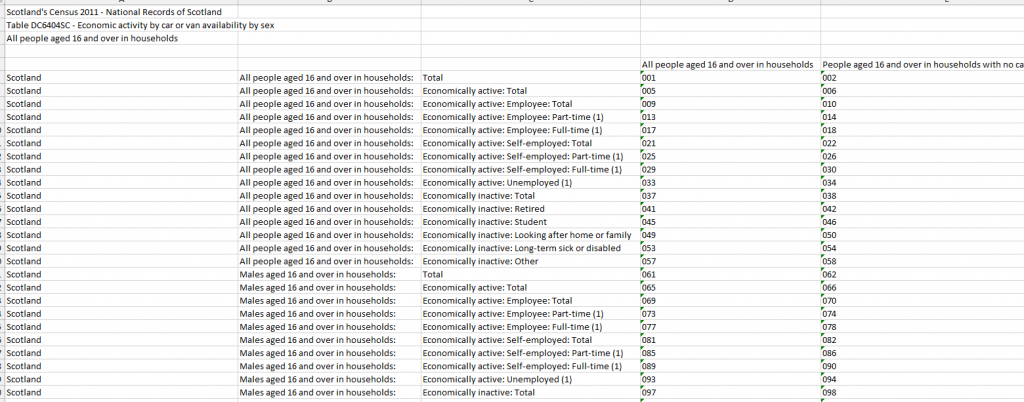
To ensure that we captured all the information to comprehensively describe each cell, we had to cross check between the csv description files, the table layout files, and the headers and footers files, which was very time-consuming, but needed to be done. We discovered during QA process that the table layouts didn’t necessarily contain all the information required, which necessitated altering our working model as well as reprocessing a large batch of data with the associated changes.
In terms of numbers of cells, for Northern Ireland there were approximately 140,000 cells, so similar numbers to England Wales. For Scotland there were approximately 40,000 cells. Ordinarily the presumption would be that to process the Scottish data, it should have been easier as there are less metadata to process but, due to the issues highlighted above, this didn’t prove to be the case.
For the Scottish data, there were more value judgements to determine if the same concept was being described. This then made processing the data a very lengthy task but also had a knock-on effect in the QA stages because the person performing the QA of the data needed to confirm that the value judgement made sense and they needed to independently follow the logic to determine if the concept was the same or different. This necessitated team discussions to reach a consensus or if further investigation was needed. The results of these discussions could mean going back to previously described data to check that the new theory held true with the possibility of refactoring work.
We originally processed and loaded into InFuse the majority of ONS data, then performed a subsequent data release which consisted of the Northern Irish and Scottish data, owing to the overheads of having to retrospectively go back and amend the working model when things were identified as needing change. As it was, it was possible to identify all the places which contained the concepts potentially needing change and check to ensure that all the data being described was consistent.
Ideally we would have waited until all the data had been released by the agencies before beginning processing to reduce the numbers of changes we had to make to our working model. This would have meant that we would have been better placed to look at all of the data to see how best to describe the concepts. However, we wanted to release the data as soon as possible to allow our users to access it.
Once we had all the cells described in a consistent way, it was then possible to match this metadata from Scotland and Northern Ireland into the existing set formed when the ONS data was processed, thus creating a UK dataset, with exceptions where the concepts described were country specific.
This matching allowed us to identify duplicates within the dataset. We then analysed the associated data tables for each of the tables in the collection to work out for what geographic coverage and granularity the data was available. We combined this information with the list of the datasets to determine where we needed to append the data together to create composite data tables containing values from across the UK.
One data processing step before this appending exercise was to make sure we maximised the value of the raw data by appending the separate parts of the data tables together. Typically, each data table is supplied in separate files per geography type and so, using our UK geography hierarchy model, we aggregated the data up to fill any gaps in the data supplied. We ensured that we only did this for data which are ‘safe’ to aggregate and therefore non-disclosive.
We did run into an issue when we loaded the data as it wasn’t always clear what the use of dashes meant within the data files. Sometimes ‘–’ was used to indicate an impossible cell, e.g. Married people age 0 to 4, which would then make a data value of null. In other cases ‘–’ was used to indicate that there could be a value but for some reason one wasn’t supplied. The use of the ‘–’ meant that we had to do some preprocessing of the data files to enable us to load the data into our system, where we had told it that the cell contents should be a number.
During this data aggregation step, we identified some further challenges with data from Scotland. The aggregated data values weren’t matching the figures for Council Areas or the country total. On investigation, this was because Scotland released their data at Super Output Area equivalent using 2001 definitions. Due to changes in the makeup of the Council areas between 2001 and 2011, some of the data was either being undercounted or overcounted. Luckily around this time in the process, Scotland rereleased their data using the newly created 2011 Super Output Areas for Scotland. We were then able to swap out the 2001 Super Output Area data with the 2011 Super Output Area data and rerun the data aggregation exercise, which greatly reduced the inconsistency of data. This then highlighted a number of cells where the data had been corrected, so we needed to also swap out the Scotland totals.
Once this data work was complete, we were in a position to load the metadata into our InFuse application, which gave us the opportunity to see the implications of some of our earlier decisions.

Richard Wiseman, Data Sherpa on the team says:
“We identified an issue with how we had treated ‘Economic activity’. This codelist had doubled in size between our previous release (which primarily contained ONS data) and this new release. The larger codelist now contained about 200 codes. This was due to erring on the side of caution when we described the data. We decided to investigate this to see if we could normalise this codelist further, as we knew from our download logs that it is the Economic activity codelist most often downloaded by our users.
During this investigation, we discovered an issue to do with whether students were counted as economically active or inactive. We followed these through by looking in detail at the data to determine whether the numbers were the same even if we’d opted to describe something slightly differently. We discovered that in a lot of instances, this was in fact the case, which meant we could reduce the numbers of codes used. We also decided to reorganise the code hierarchies to make it more explicit for our users to see whether the figures included students or not. This then had a knock-on effect in that we were able to match more data, which then meant we needed to redo the append step creating new versions of our composite UK tables.”
What next?
Our data platform InFuse was originally developed with data from England and Wales and loading additional rich data from Scotland and Northern Ireland exposed some limitations of the application. The application’s logic presumed that data was available across all the countries, but from Table 3 shown above this is no longer the case, so when using InFuse it seemed that you could get the data from across the UK, which then resulted in blank cells for some of the geographic areas selected. To address this issue we have created a version of InFuse where users can define the geography areas that they’re interested in and then the wizard will filter the topics or categories available based on that selection.
We have also started extending our engagement with existing and future users of our data and resources to help us inform future developments of our UK census data interface.